What is a model?

Before delving into the basic components of Stable Diffusion, let’s briefly touch on what a model is for those who haven’t used software that incorporates AI. Feel free to skip this section if you’re already familiar with the concept. In AI, a model is essentially a set of learned rules that transform input into output. For example, in a photo editing app, a model might take an image as input and enhance its colors, resulting in a new output image. Typically, this model is stored as one or more files on a computer disk. Understanding this concept will help in grasping how Stable Diffusion functions.

Let’s consider a simple example to understand how models work. Imagine you’re dealing with two friends.

First friend: “Your other friend will show up here soon. When he is here, can you sum any two numbers he gives you?”

You: “Sure”

Then, the second friend comes.
Second friend: “Two numbers are 10 and 100. “

Without hesitation, you add them up and say, ‘That’s easy, it’s 110.’

Congratulations! In this scenario, you’ve just acted like a model! Here’s what you did:

• You understood the the rule to apply is the rule of addition.
• You received inputs (10 and 100).
• You applied the addition rule to these inputs.
• Finally, you output the result (110).

This process is akin to how a computer model operates, given that it has already learned beforehand rules to apply when inputs are given. This is called inference or prediction. However, in the case of computers, learning these rules often involves training on extensive data sets to understand patterns or calculations. So, how do we teach these complex rules to a computer? That’s where machine learning comes in.

For those of you who have written computer code but haven’t used a model, this sounds exactly like getting a computer to do what you want by writing code. What’s the difference? That’s a very valid question. Let me illustrate the difference with another example. Imagine the following conversation:

Friend: “I’ll give you three numbers. Your task is to figure out how I came up with the third number from the first and second numbers.”

You: “OK. Go ahead.“

Friend: “Here’s the first set: 10, 8, and 2.”

You: “Hmm, I have an idea, but I’d like another example to be sure.”

Friend: “Sure thing. Here’s another: 20, 5, and 15.”

You: “Ah, that’s easy! You’re subtracting the second number from the first.”

Friend: “Exactly, you got it right!”

Let’s reflect on what just happened:

• You were given two examples of input and output.
• From these, you deduced the rule to convert the input to the output. This process is akin to one way of training a model in machine learning, known as supervised learning. In our example, the first two numbers are the inputs, each referred to as a feature, and the third number is the output, known as the label.

Now, you might wonder how a computer program can learn rules from examples to build a model. I’ll delve into that in the next section, but first, it’s important to note that unlike the simple rule we observed here, most models involve many more rules, especially as we increase the number of features. Consequently, we need a vast number of examples to accurately deduce these rules. Take Stable Diffusion, for instance; it was trained with billions of examples.”

Rule Itself vs Values Used in the Rule

Understanding the distinction between the rules applied and the set of values used in these rules is crucial in machine learning.

Consider these examples where you’re given a set of numbers:

$10.00, $1.00
$ 9.00, $0.90
$ 8.00, $0.80

As a model, you might quickly deduce that the second column represents a sales tax calculated by multiplying the first number by 10%. This assumption is valid.

Now, look at a different set:

$10.00, $2.00
$ 9.00, $1.80
$ 8.00, $1.60

Here, you, acting as a model, might realize that the tax rate has changed to 20%.

What’s the key difference between these two scenarios?
In both cases, you’re using multiplication on the first number, but the values (percentages) used for multiplication differ. The rule – multiplication – remains constant, but the values used in this rule vary. This distinction is fundamental to understanding how a model operates.

In a typical model, the rules themselves (e.g., the manner and frequency of input processing and reprocessing) are predetermined by the model’s human designer. During training, using this set of rules, the model is exposed to numerous examples, and the values (or weights) to be used in these rules are determined. In machine learning terminology, these rules are called the ‘architecture’. In neural networks, each rule is referred to as a ‘layer’, and the values used in the rules are known as ‘weights’.

A point of confusion can arise when saving a model: it can be saved with or without its architecture, though the weights are always saved. So, when you want to use a model that only contains weights, you need to reconstruct the architecture, which embodies the actual rules.

In machine learning models, input features often undergo transformations through a series of rules. These transformations modify the input value in various ways, depending on the applied rules. Here are some common rules used in models:

• Weighted Summation: Multiply each input by a different number (known as a weight) and sum up these results. This process effectively alters the original feature values based on the weights.
• Summation with Bias: Similar to the first rule, but includes an additional step of adding another number (often referred to as a bias) to the sum. This can shift the output value in a desired direction, providing more flexibility to the model.
• Rectified Linear Unit (ReLU): If the input is less than 0, set the result to 0; if it is 0 or above, retain the feature value as is. This rule, commonly known as ReLU in neural networks, introduces non-linearity, allowing the model to handle complex patterns more effectively.
• Transformation to a Range: Apply a mathematical transformation to an input so that its value falls within a specific range, often 0 to 1. This could be through normalization or other functions like the sigmoid, which is especially useful in contexts like binary classification or when outputs need to be bounded.
• Pixel Analysis for Images: In image processing models, analyze the values of surrounding pixels to determine the optimal combination for an output. This rule is essential in capturing patterns in image data.

Let’s go over how a model learns the right weight. I’m using a toy example. You are shown the following numbers.

I’m using the following per the convention:

x: input
y: label
w: weight
y_hat: your prediction (which is w times x, or w * x)

x, y
1, 10
2, 20
3, 30

The goal is to figure out how to convert the feature on the first column to the label in the second column. As human, you would instantly know that the right answer may be multiply by 10. So the weight should be 10. But how would a model know? Let’s say that you as a model design design the architecture that the right answer should be apply multiplication only once with the unknown weight.

The first step is to pick some number as the guess which is oftentimes a random number in the real world model. Let’s pick 2.

Then the next step is compute the output using your guess.

x * w = y_hat
1 * 2 = 2
2 * 2 = 4
3 * 2 = 6

Now your initial output is very off, but you go ahead and compute how off this result is from the actual label is.

y - y_hat = difference
10 - 2 = 8
20 - 4 = 16
30 - 6 = 24

However, there is one more twist to this. Since difference can be measured objectively even when the your output is bigger than the label (e.g. your output is 100 when the label is 10), it is customary to square the difference (In below, I’m using the “^2” sign to mean to square the number). To compute the per example loss, let’s divide by the number of examples.

(8^2 + 16^2 + 24^2) / 3 = 298.66

What if your initial guess is completely right and use 10 as the weight? Would would be the loss?

The answer is 0. Because feature x your guess completely matches for each label, so there won’t be any difference.

The goal of model training is to tweak the weight so that the loss is reduced, and ideally as close to 0 as possible.

Then how will the model training code adjust the weight? We already know that the correct weight is 10, and we estimated 2, so it’s obvious that if we increase the weight, loss should decrease, right?

Then, how would the training code know that increasing the weight is the way to go?

Here comes the knowledge of calculus that you may have learned in high school would come into help, but you may not have taken the calculus class, so let’s go over the basics. What we want to know is how we can adjust the weight in such a way that changing the weight will reduce loss. What calculus tells us is that if we take a look at an extremely small change in the value of weight, we will know how the loss will change and gives us the equation for that.

Use y for the label, x for the feature and w for the weight, as it turns out that the change of loss with respect to the small change in weight is given by the following:

-2 * x * y + 2 * x^2 * w

This is called the gradient.

Since we have three examples of x (1, 2, 3). We will need to compute this value for each of x, then add them up and divide by 3 to compute the mean gradient.

Let’s plug in numbers.

For x=1, g = -2 * x * y + 2 * x^2 * w = - 2 * 1 * 10 + 2 * 1^2 * 2 = -16
For x=2, g = -2 * x * y + 2 * x^2 * w = - 2 * 2 * 20 + 2 * 2^2 * 2 = -64
For x=3, g = -2 * x * y + 2 * x^2 * w = - 2 * 3 * 30 + 2 * 3^2 * 2 = -144

Mean gradient = -74.66

What does this mean? This means that if we increase the value of w a little bit, then the loss would go down. Since calculus tells us that this relationship is valid only for a super small change in w, let’s increase the value of w a little bit. The common way to do so is to subtract a small portion of gradient from the weight,which is the same thing. Let’s take 1% of the gradient and subtract from w.

Then:

New weight = w - (-74.66/100) = w + 74.66/100 = w + 0.7466 = 2.7466 

The idea is to keep repeating this step until the loss is close to 0 or won’t go down further. Shown below is the output of the Python (a programming language) code to compute the loss as I did more iterations. Epoch is a unit to refer to the processing done for the entire dataset, which in this case is 3 as there are only 3 examples.

Epoch: 0001, w:2.7466666666666666, loss: 298.6666666666667
Epoch: 0002, w:3.4236444444444443, loss: 245.51727407407407
Epoch: 0003, w:4.037437629629629, loss: 201.82611116773668
Epoch: 0004, w:4.593943450864197, loss: 165.91003342926476
Epoch: 0005, w:5.098508728783539, loss: 136.38542125811915
Epoch: 0006, w:5.555981247430409, loss: 112.11487784845207
Epoch: 0007, w:5.970756331003571, loss: 92.16341247488754
Epoch: 0008, w:6.346819073443237, loss: 75.76242120602309
Epoch: 0009, w:6.687782626588535, loss: 62.280077450071246
Epoch: 0010, w:6.996922914773605, loss: 51.1969916674008
...
Epoch: 0068, w:9.989778135013104, loss: 0.0005931598724093081
Epoch: 0069, w:9.990732175745215, loss: 0.0004876037777815344
...
Epoch: 0350, w:9.999999999999991, loss: 5.301145283085199e-28
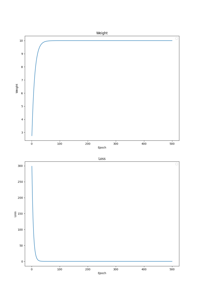
Epoch: 0351, w:9.999999999999991, loss: 4.00741339852274e-28

Note that at the 10th iteration, w is still roughly 7 and is lower than the expected target which is 10, and it took 69 iterations to reach 9.99 which is pretty close. At 351th iteration, loss is effectively 0 and w is effectively 10, so we can call it done. Below plot is a visualization to show how loss and weight change over multiple iterations.