Text Embedding Generator

Unless you’re already familiar with machine learning or natural language processing, the term ’embedding’ might seem obscure, and its underlying concept somewhat elusive. To demystify this, I’ll provide a conceptual overview of embedding in this section. If you’re already versed in embeddings, feel free to skip ahead.

Consider an analogy involving a conversation between two friends engaged in a game. The rules of the game are simple:

1. Choice of Numbers: Each player picks two numbers, both of which range from 0 to 1.
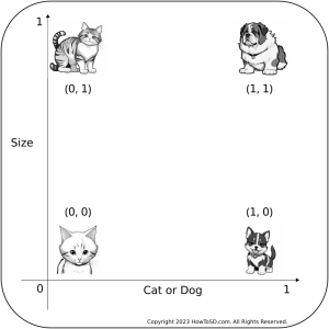
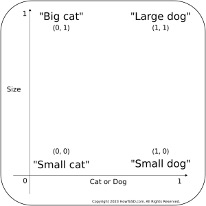
2. Number Representations: The first number signifies an animal – ‘0’ for a cat and ‘1’ for a dog. The second number denotes size – ‘0’ for small and ‘1’ for big.

You can see the below figure to get an idea. For instance, selecting the numbers 1 and 0 would correspond to a dog and the size is small, so it means a small dog. Once chosen, you jot these numbers down on a piece of paper and proceed to draw the animal as per your selection. The game’s crux lies in your friend’s attempt to deduce the numbers you chose based solely on your drawing.

Let’s actually play a few games to solidify your understanding. I’ll show you the drawing I made using Stable Diffusion and you will guess the two numbers I have in mind.

Here is the first one:

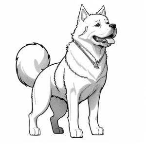
If you guessed (1, 0.8), you won.

Here is the second one.

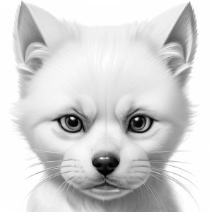
This one is actually hard. I intentionally generated an image that is kinda cat and kinda dog. So the numbers I had in mind was (0.5, 0.2) meaning a cross between a dog and a cat, and the size is on the small side.

The central lesson from our game is the possibility of mapping images of animals onto a coordinate system based on certain attributes — in our case, animal type and size. The set of coordinate points assigned to each image carries specific meanings. For instance, a value of 0.5 for the first number could indicate an animal that’s a mix between a dog and a cat. We’ve used only two numbers here, but what happens if we use more? Can we capture more characteristics? The answer is yes, and that’s the essence of embedding. The numbers that represent an image or an object in this way are known as an ’embedding.’

However, there’s a crucial aspect to be aware of. This mapping of an image to a set of numbers is accomplished using machine learning, and the resulting embedding might not be organized as a human would naturally do it. For example, while a human might arrange the numbers with the first representing animal type and the second indicating size, a machine learning model is likely to arrange these numbers in a completely different manner. Therefore, a single number might not neatly correspond to a concept like the size of an animal.

So far, we’ve discussed embeddings in the context of images, but this concept applies equally to text. Figure 7 below provides an example of this. The only difference is that each point now represents words describing the animal type and size, instead of images. The task is to train a model that converts words to corresponding numerical values. For instance, the phrase ‘Large dog’ might be converted to (1, 1). Similarly, a point like (0.5, 1) could be translated to ‘Medium-sized dog’ in English. How to train such a model is a complex topic beyond the scope of this discussion, but there are various methods. In the next section, I will briefly outline the method used in training a specific text embedding model employed in Stable Diffusion.

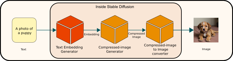
In the previous section, we explored how words can be mapped to coordinates in a multi-dimensional space, with these coordinates being referred to as an ’embedding.’ In the case of Stable Diffusion, the text input you provide undergoes a transformation into such an embedding before being processed by the compressed-image generation model.

Let’s explore an intriguing aspect of Stable Diffusion, particularly the model it uses for generating text embeddings. This model is known as the CLIP ViT-L/14 text encoder [1]. For those with a background in computer programming, you can examine the source code (specifically at line 137) to see how this setup is implemented. It’s noteworthy that the developers of Stable Diffusion didn’t train this model themselves. Instead, it was developed and trained by OpenAI, the creators of the widely recognized ChatGPT.

Stable Diffusion leverages this model to transform text or prompts into text embeddings. Interestingly, you can access and download the model from Hugging Face’s CLIP-ViT-L/14 repository. Link to the paper is listed in the reference section [2].

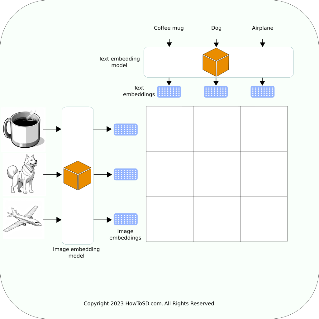
A notable feature of this model is its dual functionality: it contains two internal components. One is designed to generate embeddings from images, while the other focuses on generating embeddings from text. In the context of Stable Diffusion, specifically for text-to-image generation, the text-based component is utilized.

Regarding its training methodology, the model was exposed to a vast array of image-text pairs. During this training process, the text embeddings generated for a given text are compared against the image embeddings of the corresponding image, as well as against embeddings from non-matching images. To visualize this, consider the following example: in the figure below, you might be asked to compare the text embedding of a coffee mug with the image embedding of a coffee mug. If they align, you mark it with a check. If not, it’s marked with an “x”. This comparative process is repeated across all the pairs.

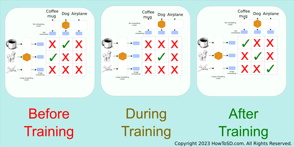
The figure below illustrates the scoring evolution across different phases of training. Initially, on the left, the two models lack the knowledge to generate accurate embeddings. This inaccuracy is evident when comparing embeddings: for instance, the image embedding of a coffee mug and the text embedding of the word ‘dog’ are mistakenly similar. Similarly, the image embedding of a dog and the text embedding of ‘coffee mug’ are incorrectly aligned. Moreover, none of the embedding pairs that should match are actually matching.

Thankfully, there’s a mathematical method to quantify the closeness of these matches. Once the training program calculates this metric, it can adjust the model parameters accordingly. The middle figure represents a typical scenario post-adjustment. Now, the image embedding of a dog correctly matches the word ‘dog,’ but there are still mismatches with other pairs like ‘coffee mug’ and ‘airplane.’

With continuous feedback during training, the model undergoes further refinements. Eventually, as shown in the figure on the right, the model achieves the desired outcome. At this stage, embeddings generated for both text and images have meaningful representations within the multi-dimensional space, accurately reflecting the intended correlations.
In machine learning, the process I described is known as contrastive learning, or more specifically, contrastive pre-training. This is precisely what ‘CLIP’ stands for – Contrastive Language-Image Pre-training, highlighting its focus on learning from contrasts between language (text) and images.

Have you ever wondered about the number of numerical values involved in representing text in the CLIP model used by Stable Diffusion? For the standard version of this model, the number is a staggering 59,316. This total is the result of 77 elements, each composed of 768 numbers (77 x 768 = 59,316). To truly appreciate the magnitude of this, let’s recall the simpler example we discussed earlier, which utilized merely two numbers. The scale we’re examining here is roughly 30,000 times larger than that!

This expansive array of numbers in the CLIP model allows for the incredibly detailed and nuanced representation of textual information. It’s a prime example of how advanced machine learning models like CLIP can process and interpret vast quantities of data, far beyond the capabilities of simpler, less sophisticated systems.

This immense complexity enables Stable Diffusion to capture and process a vast array of nuances in the text, leading to more accurate and detailed image generation.

Up to this point, we have explored how the text embedding generator in Stable Diffusion converts input text into embeddings. However, there’s a crucial preliminary step in this process that often goes unnoticed because it operates ‘under the hood.’ As a user, you might not see this directly, but understanding it can be beneficial. The transformation from text to an embedding occurs in two distinct phases:

1. Tokenization: This is the process of breaking down the text into smaller units, known as tokens.
2. Token to Embedding Conversion: This step, carried out by the text embedding model, involves converting these tokens into numerical embeddings.

It’s important to note that another module, often referred to as a tokenizer, is responsible for the tokenization phase.

Generally, machine learning models do not process words or strings directly. Instead, they require a preceding module to convert these textual elements into numerical values, which are then fed into the model. Typically, integers are used in this conversion process, rather than floating-point numbers.

To illustrate this with a concrete example, consider the sentence: ‘A puppy is running in the yard.’ During tokenization, this sentence is broken down into the following individual tokens.

[Token index] Token ID Token
[0] 49406 <|startoftext|>
[1] 320 a
[2] 6829 puppy
[3] 533 is
[4] 2761 running
[5] 530 in
[6] 518 the
[7] 4313 yard
[8] 269 .
[9] 49407 <|endoftext|>
... 10 to 75 omitted as they are all <|endoftext|>
[76] 49407 <|endoftext|>

You can explore the token-to-number mapping used by the CLIP model at Hugging Face. For instance, the word ‘puppy’ is assigned the number 6829 in this mapping. A few important notes:

Special Tokens: Tokens like <|startoftext|> and <|endoftext|> are special markers used by the tokenizer. They are not part of the original text but are crucial for indicating the beginning and end of the text input.

Limited Vocabulary Size: The total number of unique words in this tokenizer’s mapping is 49,408. While this number is significant, it might seem insufficient to cover every word in the English language. What happens when you input a sentence containing words not in the tokenizer’s vocabulary? Let’s test with the sentence: ‘HowToSD.com is a great website.’

[0] 49406 <|startoftext|>
[1] 38191 howto
[2] 4159 sd
[3] 269 .
[4] 2464 com
[5] 533 is
[6] 320 a
[7] 830 great
[8] 3364 website
[9] 269 .
[10] 49407 <|endoftext|>
... (rest omitted)

In this example, ‘HowToSD.com’ is split into ‘howto’, ‘sd’, ‘.’, and ‘com’. This segmentation is effective and reflects the logic behind the naming of the website. Even if longer words are broken into smaller tokens, which might not represent the original English word accurately, this can still be effective. The key is the mapping of these combinations to images, which is crucial in the context of Stable Diffusion. The substantial size of the training dataset used by the Stable Diffusion team likely includes these token combinations, facilitating accurate image generation.

Token Limitation and Solutions: An observant reader might question the token limit, noticing that there appear to be 77 tokens, each seemingly mapping to a word or part of a word. Does this imply Stable Diffusion can only use a maximum of 77 words in a prompt? Initially, the original Stable Diffusion model was limited to 75 words at most due to the start and end text tokens. However, third-party adaptations like automatic1111 have developed workarounds to this limitation, expanding the potential for more extended text inputs.

[1] Computer Vision and Learning research group at Ludwig Maximilian University of Munich. Stable Diffusion. Retrieved from https://github.com/CompVis/stable-diffusion.
[2] Alec Radford et al. Learning Transferable Visual Models From Natural Language Supervision. Retrieved from https://arxiv.org/abs/2103.00020.